Plot a fitted rgcca permutation object. The set of candidate tuning parameters are represented on the y-axis and the RGCCA objective function - obtained from both the original and permuted blocks - on the x-axis. If type = "zstat" the value of the zstat for the various parameter sets are reported on the x-axis.
Usage
# S3 method for permutation
plot(
  x,
  type = "crit",
  cex = 1,
  title = NULL,
  cex_main = 14 * cex,
  cex_sub = 12 * cex,
  cex_point = 3 * cex,
  cex_lab = 12 * cex,
  display_order = TRUE,
  show_legend = FALSE,
  ...
)
Arguments
- x
A fitted rgcca_permutation object (see
rgcca_permutation).- type
A string indicating which criterion to plot. Default is 'crit' for the RGCCA criterion. Otherwise, the pseudo Z-score is used.
- cex
A numeric defining the size of the objects in the plot. Default is one.
- title
A string specifying the title of the plot.
- cex_main
A numeric defining the font size of the title. Default is 14 * cex.
- cex_sub
A numeric defining the font size of the subtitle. Default is 12 * cex.
- cex_point
A numeric defining the font size of the points. Default is 3 * cex.
- cex_lab
A numeric defining the font size of the labels. Default is 12 * cex.
- display_order
A logical value for ordering the variables. If TRUE, variables are ordered from highest to lowest absolute value. If FALSE, the block order is used. Default is TRUE.
- show_legend
A logical value indicating if legend should be shown (default is FALSE).
- ...
Additional graphical parameters.
Examples
data(Russett)
A <- list(
agriculture = Russett[, seq(3)],
industry = Russett[, 4:5],
politic = Russett[, 6:11]
)
perm_out <- rgcca_permutation(A, par_type = "tau",
n_perms = 2, n_cores = 1,
verbose = TRUE)
print(perm_out)
#> Call: method='rgcca', superblock=FALSE, scale=TRUE, scale_block=TRUE, init='svd',
#> bias=TRUE, tol=1e-08, NA_method='na.ignore', ncomp=c(1,1,1), response=NULL,
#> comp_orth=TRUE
#> There are J = 3 blocks.
#> The design matrix is:
#> agriculture industry politic
#> agriculture 0 1 1
#> industry 1 0 1
#> politic 1 1 0
#>
#> The factorial scheme is used.
#>
#> Tuning parameters (tau) used:
#> agriculture industry politic
#> 1 1.000 1.000 1.000
#> 2 0.889 0.889 0.889
#> 3 0.778 0.778 0.778
#> 4 0.667 0.667 0.667
#> 5 0.556 0.556 0.556
#> 6 0.444 0.444 0.444
#> 7 0.333 0.333 0.333
#> 8 0.222 0.222 0.222
#> 9 0.111 0.111 0.111
#> 10 0.000 0.000 0.000
#>
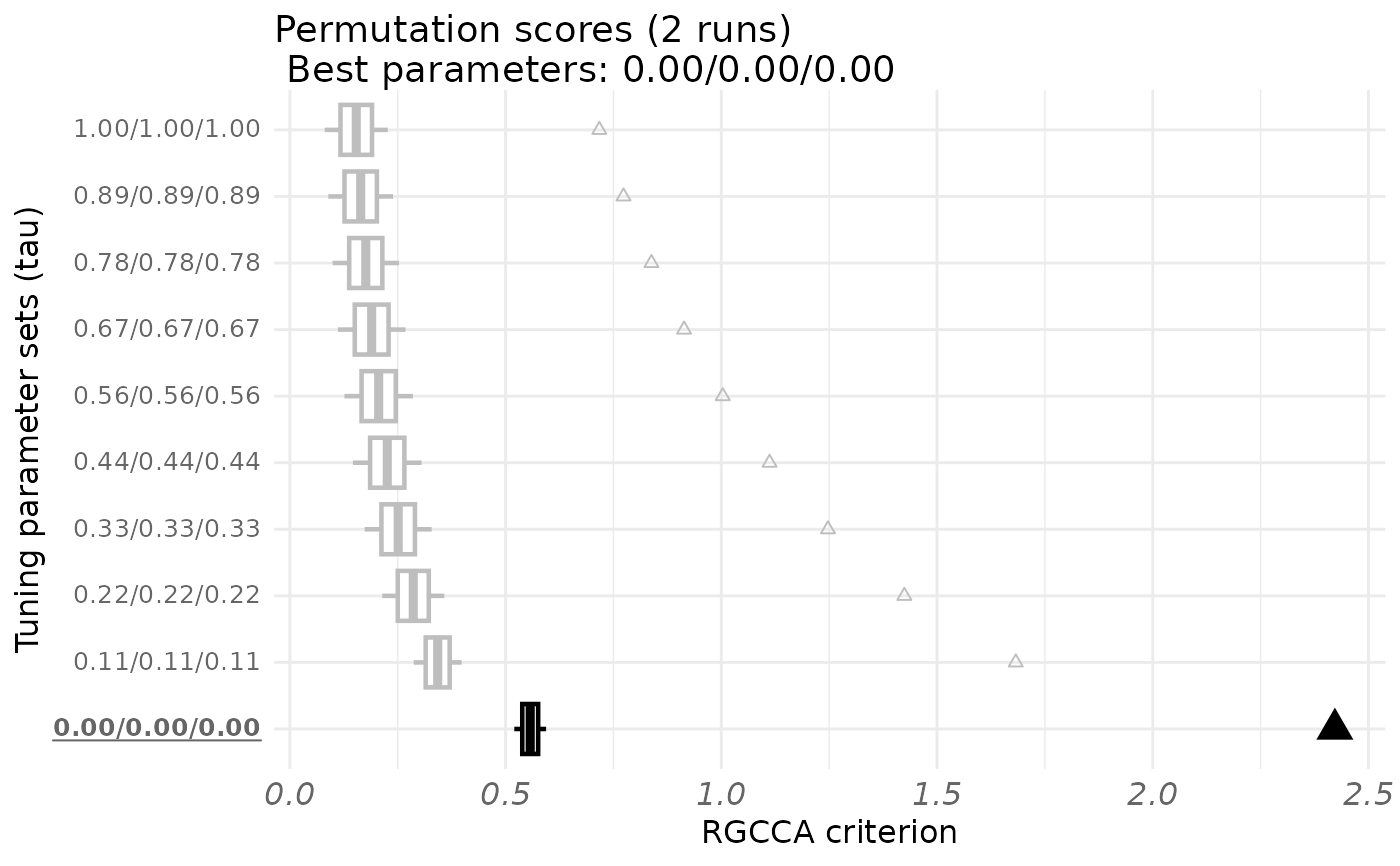
#> Tuning parameters Criterion Permuted criterion sd zstat p-value
#> 1 1.00/1.00/1.00 0.717 0.154 0.1033 5.45 0
#> 2 0.89/0.89/0.89 0.773 0.164 0.1061 5.74 0
#> 3 0.78/0.78/0.78 0.838 0.176 0.1086 6.09 0
#> 4 0.67/0.67/0.67 0.914 0.190 0.1108 6.53 0
#> 5 0.56/0.56/0.56 1.003 0.206 0.1123 7.10 0
#> 6 0.44/0.44/0.44 1.112 0.226 0.1124 7.89 0
#> 7 0.33/0.33/0.33 1.247 0.251 0.1098 9.07 0
#> 8 0.22/0.22/0.22 1.424 0.286 0.1016 11.20 0
#> 9 0.11/0.11/0.11 1.682 0.343 0.0786 17.04 0
#> 10 0.00/0.00/0.00 2.422 0.557 0.0521 35.80 0
#> The best combination is: 0.00/0.00/0.00 for a z score of 35.8 and a p-value of 0.
plot(perm_out)
 perm.out <- rgcca_permutation(A,
par_type = "sparsity",
n_perms = 5, n_cores = 1,
verbose = TRUE
)
print(perm.out)
#> Call: method='sgcca', superblock=FALSE, scale=TRUE, scale_block=TRUE, init='svd',
#> bias=TRUE, tol=1e-08, NA_method='na.ignore', ncomp=c(1,1,1), response=NULL,
#> comp_orth=TRUE
#> There are J = 3 blocks.
#> The design matrix is:
#> agriculture industry politic
#> agriculture 0 1 1
#> industry 1 0 1
#> politic 1 1 0
#>
#> The factorial scheme is used.
#>
#> Tuning parameters (sparsity) used:
#> agriculture industry politic
#> 1 1.000 1.000 1.000
#> 2 0.953 0.967 0.934
#> 3 0.906 0.935 0.868
#> 4 0.859 0.902 0.803
#> 5 0.812 0.870 0.737
#> 6 0.765 0.837 0.671
#> 7 0.718 0.805 0.605
#> 8 0.671 0.772 0.540
#> 9 0.624 0.740 0.474
#> 10 0.577 0.707 0.408
#>
#> Tuning parameters Criterion Permuted criterion sd zstat p-value
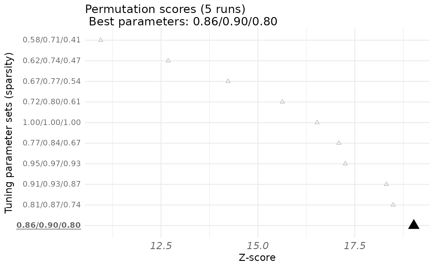
#> 1 1.00/1.00/1.00 0.717 0.0872 0.0381 16.5 0
#> 2 0.95/0.97/0.93 0.680 0.0826 0.0346 17.3 0
#> 3 0.91/0.93/0.87 0.640 0.0768 0.0308 18.3 0
#> 4 0.86/0.90/0.80 0.588 0.0698 0.0272 19.0 0
#> 5 0.81/0.87/0.74 0.502 0.0620 0.0238 18.5 0
#> 6 0.77/0.84/0.67 0.409 0.0536 0.0208 17.1 0
#> 7 0.72/0.80/0.61 0.324 0.0450 0.0179 15.6 0
#> 8 0.67/0.77/0.54 0.251 0.0360 0.0151 14.2 0
#> 9 0.62/0.74/0.47 0.188 0.0285 0.0126 12.7 0
#> 10 0.58/0.71/0.41 0.136 0.0232 0.0103 10.9 0
#> The best combination is: 0.86/0.90/0.80 for a z score of 19 and a p-value of 0.
plot(perm.out, type = "zstat")
perm.out <- rgcca_permutation(A,
par_type = "sparsity",
n_perms = 5, n_cores = 1,
verbose = TRUE
)
print(perm.out)
#> Call: method='sgcca', superblock=FALSE, scale=TRUE, scale_block=TRUE, init='svd',
#> bias=TRUE, tol=1e-08, NA_method='na.ignore', ncomp=c(1,1,1), response=NULL,
#> comp_orth=TRUE
#> There are J = 3 blocks.
#> The design matrix is:
#> agriculture industry politic
#> agriculture 0 1 1
#> industry 1 0 1
#> politic 1 1 0
#>
#> The factorial scheme is used.
#>
#> Tuning parameters (sparsity) used:
#> agriculture industry politic
#> 1 1.000 1.000 1.000
#> 2 0.953 0.967 0.934
#> 3 0.906 0.935 0.868
#> 4 0.859 0.902 0.803
#> 5 0.812 0.870 0.737
#> 6 0.765 0.837 0.671
#> 7 0.718 0.805 0.605
#> 8 0.671 0.772 0.540
#> 9 0.624 0.740 0.474
#> 10 0.577 0.707 0.408
#>
#> Tuning parameters Criterion Permuted criterion sd zstat p-value
#> 1 1.00/1.00/1.00 0.717 0.0872 0.0381 16.5 0
#> 2 0.95/0.97/0.93 0.680 0.0826 0.0346 17.3 0
#> 3 0.91/0.93/0.87 0.640 0.0768 0.0308 18.3 0
#> 4 0.86/0.90/0.80 0.588 0.0698 0.0272 19.0 0
#> 5 0.81/0.87/0.74 0.502 0.0620 0.0238 18.5 0
#> 6 0.77/0.84/0.67 0.409 0.0536 0.0208 17.1 0
#> 7 0.72/0.80/0.61 0.324 0.0450 0.0179 15.6 0
#> 8 0.67/0.77/0.54 0.251 0.0360 0.0151 14.2 0
#> 9 0.62/0.74/0.47 0.188 0.0285 0.0126 12.7 0
#> 10 0.58/0.71/0.41 0.136 0.0232 0.0103 10.9 0
#> The best combination is: 0.86/0.90/0.80 for a z score of 19 and a p-value of 0.
plot(perm.out, type = "zstat")